

Java programmers use data structures to store and organize data, and we use algorithms to manipulate the data in those structures. The more you understand about data structures and algorithms, and how they work together, the more efficient your Java programs will be.
This tutorial launches a short series introducing data structures and algorithms. In Part 1, you’ll learn what a data structure is and how data structures are classified. You’ll also learn what an algorithm is, how algorithms are represented, and how to use time and space complexity functions to compare similar algorithms. Once you’ve got these basics, you’ll be ready to learn about searching and sorting with one-dimensional arrays, in Part 2.
Data structures are based on abstract data types (ADT), which Wikipedia defines as follows:
[A] mathematical model for data types where a data type is defined by its behavior (semantics) from the point of view of a user of the data, specifically in terms of possible values, possible operations on data of this type, and the behavior of these operations.
An ADT doesn’t care about the memory representation of its values or how its operations are implemented. It’s like a Java interface, which is a data type that’s disconnected from any implementation. In contrast, a data structure is a concrete implementation of one or more ADTs, similar to how Java classes implement interfaces.
Examples of ADTs include Employee, Vehicle, Array, and List. Consider the List ADT (also known as the Sequence ADT), which describes an ordered collection of elements that share a common type. Each element in this collection has its own position and duplicate elements are allowed. Basic operations supported by the List ADT include:
Data structures that can implement the List ADT include fixed-size and dynamically sized one-dimensional arrays and singly-linked lists. (You’ll be introduced to arrays in Part 2, and linked lists in Part 3.)
There are many kinds of data structures, ranging from single variables to arrays or linked lists of objects containing multiple fields. All data structures can be classified as primitives or aggregates, and some are classified as containers.
The simplest kind of data structure stores single data items; for example, a variable that stores a Boolean value or a variable that stores an integer. I refer to such data structures as primitives.
Many data structures are capable of storing multiple data items. For example, an array can store multiple data items in its various slots, and an object can store multiple data items via its fields. I refer to these data structures as aggregates.
All of the data structures we’ll look at in this series are aggregates.
Anything from which data items are stored and retrieved could be considered a data structure. Examples include the data structures derived from the previously mentioned Employee, Vehicle, Array, and List ADTs.
Many data structures are designed to describe various entities. Instances of an Employee class are data structures that exist to describe various employees, for instance. In contrast, some data structures exist as generic storage vessels for other data structures. For example, an array can store primitive values or object references. I refer to this latter category of data structures as containers.
As well as being aggregates, all of the data structures we’ll look at in this series are containers.
The Java Collections Framework supports many kinds of container-oriented data structures and associated algorithms. This series will help you better understand this framework.
It’s become fairly common to use design patterns to introduce university students to data structures. A Brown University paper surveys several design patterns that are useful for designing high-quality data structures. Among other things, the paper demonstrates that the Adapter pattern is useful for designing stacks and queues. The demonstration code is shown in Listing 1.
public class DequeStack implements Stack < Deque D; // holds the elements of the stack public DequeStack() < D = new MyDeque(); >@Override public int size() < return D.size(); >@Override public boolean isEmpty() < return D.isEmpty(); >@Override public void push(Object obj) < D.insertLast(obj); >@Override public Object top() throws StackEmptyException < try < return D.lastElement(); >catch(DequeEmptyException err) < throw new StackEmptyException(); >> @Override public Object pop() throws StackEmptyException < try < return D.removeLast(); >catch(DequeEmptyException err) < throw new StackEmptyException(); >> >Listing 1 excerpts the Brown University paper’s DequeStack class, which demonstrates the Adapter pattern. Note that Stack and Deque are interfaces that describe Stack and Deque ADTs. MyDeque is a class that implements Deque .
The original code that Listing 1 is based on didn’t present the source code to Stack , Deque , and MyDeque . For clarity, I’ve introduced @Override annotations to show that all of DequeStack ‘s non-constructor methods override Stack methods.
DequeStack adapts MyDeque so that it can implement Stack . All of DequeStack ‘s method are one-line calls to the Deque interface’s methods. However, there is a small wrinkle in which Deque exceptions are converted into Stack exceptions.
Historically used as a tool for mathematical computation, algorithms are deeply connected with computer science, and with data structures in particular. An algorithm is a sequence of instructions that accomplishes a task in a finite period of time. Qualities of an algorithm are as follows:
Note that while programs may be algorithmic in nature, many programs do not terminate without external intervention.
Many code sequences qualify as algorithms. One example is a code sequence that prints a report. More famously, Euclid’s algorithm is used to calculate the mathematical greatest common divisor. A case could even be made that a data structure’s basic operations (such as store value in array slot) are algorithms. In this series, for the most part, I’ll focus on higher-level algorithms used to process data structures, such as the Binary Search and Matrix Multiplication algorithms.
How do you represent an algorithm? Writing code before fully understanding its underlying algorithm can lead to bugs, so what’s a better alternative? Two options are flowcharts and pseudocode.
A flowchart is a visual representation of an algorithm’s control flow. This representation illustrates statements that need to be executed, decisions that need to be made, logic flow (for iteration and other purposes), and terminals that indicate start and end points. Figure 1 reveals the various symbols that flowcharts use to visualize algorithms.

Consider an algorithm that initializes a counter to 0, reads characters until a newline ( n ) character is seen, increments the counter for each digit character that’s been read, and prints the counter’s value after the newline character has been read. The flowchart in Figure 2 illustrates this algorithm’s control flow.
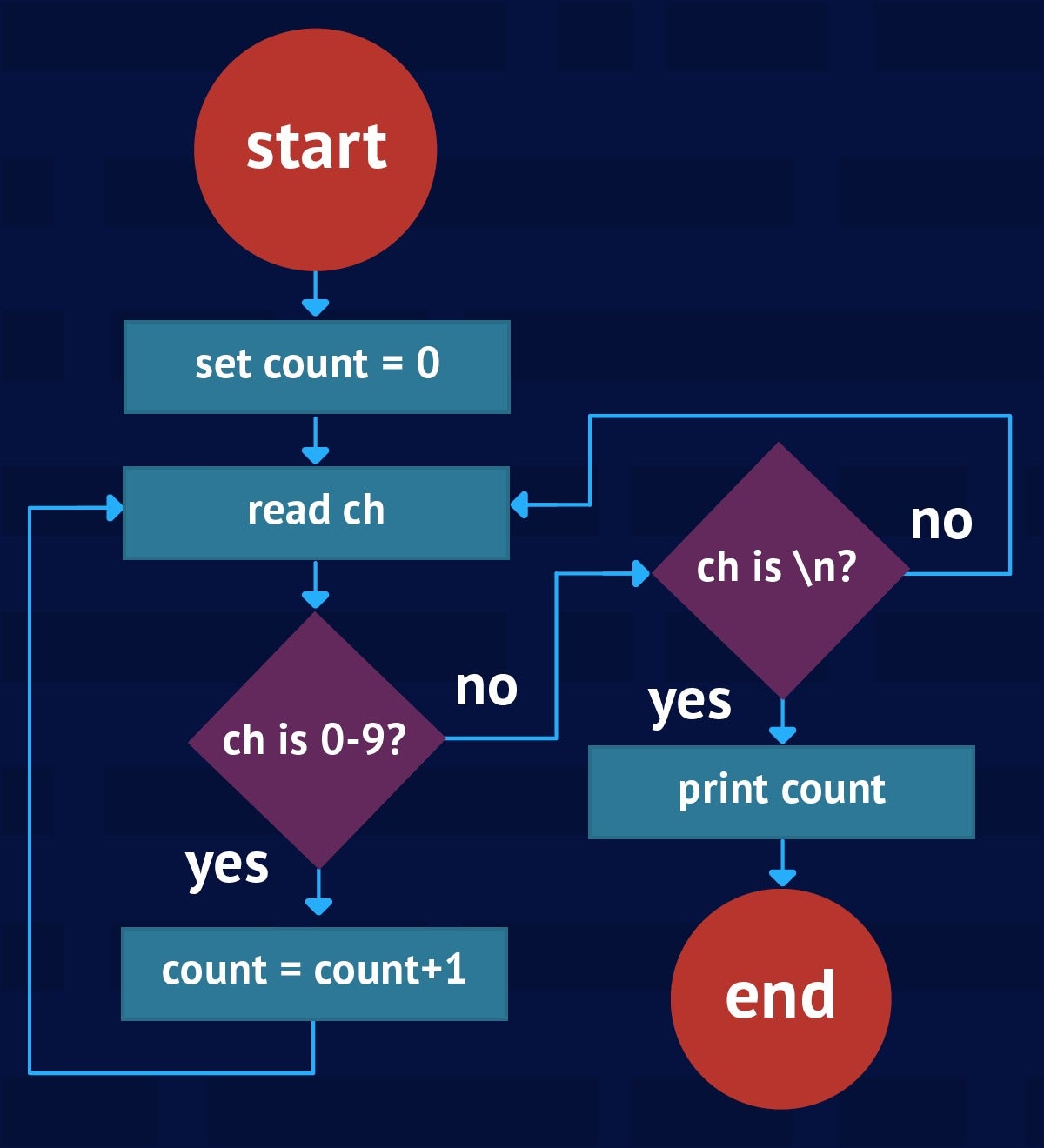
A flowchart’s simplicity and its ability to present an algorithm’s control flow visually (so that it’s is easy to follow) are its major advantages. Flowcharts also have several disadvantages, however:
An alternative to flowcharts is pseudocode, which is a textual representation of an algorithm that approximates the final source code. Pseudocode is useful for quickly writing down an algorithm’s representation. Because syntax is not a concern, there are no hard-and-fast rules for writing pseudocode.
You should strive for consistency when writing pseudocode. Being consistent will make it much easier to translate the pseudocode into actual source code. For example, consider the following pseudocode representation of the previous counter-oriented flowchart:
DECLARE CHARACTER ch = '' DECLARE INTEGER count = 0 DO READ ch IF ch GE '0' AND ch LE '9' THEN count = count + 1 END IF UNTIL ch EQ 'n' PRINT count END
The pseudocode first presents a couple of DECLARE statements that introduce variables ch and count , initialized to default values. It then presents a DO loop that executes UNTIL ch contains n (the newline character), at which point the loop ends and a PRINT statement outputs count ‘s value.
For each loop iteration, READ causes a character to be read from the keyboard (or perhaps a file–in this case it doesn’t matter what constitutes the underlying input source) and assigned to ch . If this character is a digit (one of 0 through 9 ), count is incremented by 1 .
The data structures and algorithms you use critically affect two factors in your applications:
It follows that you should be especially mindful of the algorithms and data structures you use for applications that will process lots of data. These include applications used for big data and the Internet of Things.
When choosing a data structure or algorithm, you will sometimes discover an inverse relationship between memory usage and CPU time: the less memory a data structure uses, the more CPU time associated algorithms need to process the data structure’s data items. Also, the more memory a data structure uses, the less CPU time associated algorithms will need to process the data items–leading to faster algorithm results.
As much as possible, you should strive to balance memory use with CPU time. You can simplify this task by analyzing algorithms to determine their efficiency. How well does one algorithm perform against another of similar nature? Answering this question will help you make good choices given a choice between multiple algorithms.
Some algorithms perform better than others. For example, the Binary Search algorithm is almost always more efficient than the Linear Search algorithm–something you’ll see for yourself in Part 2. You want to choose the most efficient algorithm for your application’s needs, but that choice might not be as obvious as you would think.
For instance, what does it mean if the Selection Sort algorithm (introduced in Part 2) takes 0.4 seconds to sort 10,000 integers on a given machine? That benchmark is only valid for that particular machine, that particular implementation of the algorithm, and for the size of the input data.
As computer scientist, we use time complexity and space complexity to measure an algorithm’s efficiency, distilling these into complexity functions to abstract implementation and runtime environment details. Complexity functions reveal the variance in an algorithm’s time and space requirements based on the amount of input data:
Both complexity functions are based on the size of input (n), which somehow reflects the amount of input data. Consider the following pseudocode for array printing:
DECLARE INTEGER i, x[] = [ 10, 15, -1, 32 ] FOR i = 0 TO LENGTH(x) - 1 PRINT x[i] NEXT i END
You can express the time complexity of this algorithm by specifying the time-complexity function t(n) = an+b , where a (a constant multiplier) represents the amount of time to complete one loop iteration, and b represents the algorithm’s setup time. In this example, the time complexity is linear.
The t(n) = an+b function assumes that time complexity is measured in terms of a chronological value (such as seconds). Because you’ll want to abstract machine details, you’ll often express time complexity as the number of steps to complete.
How we define a step can vary from one algorithm to another. In this case, if you identified the single print instruction as the program’s step, you would rewrite the time-complexity function in terms of the printing step:
t(n) = n ; for n array elements, n steps are needed to print the array.
It’s important to take care when defining an algorithm’s steps, so that the definition is meaningful and correlates with the algorithm’s input size. For example, it makes sense to define printing as the step for the array-printing algorithm, because printing dominates the runtime and depends on the input size (number of array elements to print).
It’s also possible to define steps in terms of comparisons and exchanges. In a sorting algorithm, for instance, you might define steps in terms of comparisons if comparisons dominate the runtime or exchanges if exchanges dominate the runtime.
It’s fairly easy to choose a time-complexity function for the array-printing example, but it can be more difficult to find this function for more complicated algorithms. Use the following rules-of-thumb to simplify this task:
These rules-of-thumb work best when a loop executes n times (where n is the size of the input data). This isn’t always the case, however, as demonstrated by the Selection Sort algorithm represented in pseudocode below:
DECLARE INTEGER i, min, pass DECLARE INTEGER x[] = [ . ] FOR pass = 0 TO LENGTH(x) - 2 min = pass FOR i = pass + 1 TO LENGTH(x) - 1 IF x[i] LT x[min] THEN min = i END IF NEXT i IF min NE pass THEN EXCHANGE x[min], x[pass] END IF NEXT pass END
Because this algorithm consists of two nested loops, you might think that its performance is quadratic. That’s only partially correct, however, because the algorithm’s performance depends on whether you choose comparisons or exchanges as the algorithm’s step:
An algorithm’s space complexity indicates the amount of extra memory needed to accomplish its task. For printing an array, a constant amount of extra memory (for code storage, stack space to store the return address when PRINT is called, and space for variable i ‘s value) is needed no matter how large the array.
You can express the array-printing algorithm’s space complexity via space-complexity function s(n) = c , where c signifies how much constant additional space is required. This value represents overhead only; it doesn’t include space for the data being processed. In this case, it doesn’t include the array.
Space complexity is expressed in terms of machine-independent memory cells instead of machine-dependent bytes. A memory cell holds some kind of data. For the array-printing algorithm, i ‘s memory cell stores an integer value.
You use time complexity and space complexity functions to compare the algorithm to others of a similar nature (one sorting algorithm to another sorting algorithm, for example). In order to ensure a fair comparison, you must use the same definition for step and memory cell in each algorithm.
Even when you have chosen identical step and memory cell definitions, however, comparing algorithms can still prove tricky. Because complexities are often nonlinear, an algorithm’s input size can greatly affect the comparison result. As an example, consider two time-complexity functions:
When n equals 1, t1 yields 25 steps, whereas t2 yields 155 steps. In this case, t1 is clearly better. This pattern continues until n equals 14, at which point t1 yields 2170 steps and t2 yields 2105 steps. In this case, t2 is the much better choice for this and successor values of n.
Computer scientists commonly compare algorithms as n tends to infinity; this is known as asymptotic analysis. Complexity functions serve as the upper bound of the algorithm’s asymptotic behavior (as n approaches infinity), and a notation called Big Oh is used to represent these upper bounds. Here’s the formal definition for Big Oh:
A function f(n) is O(g(n)) if and only if there exist two constants c and n0 such that f(n) g(n) for all n >= n0.
f(n) represents the algorithm’s computing time. When we say that this function is “O(g(n)),” we mean that (in terms of steps) it takes no longer than a constant multiplied by g(n) for this function to execute. For example, here are the Big Oh notations for the previous time-complexity functions:
You read the first equation as “t1 is order n 2 ” or “t1 is quadratic,” and read the second equation as “t2 is order n” or “t2 is linear.” The result is that you can think of time complexities as being linear, quadratic, and so on; because this is how the algorithms respond as n greatly increases.
It’s common to throw away all terms except the largest and any constant multiplier for the largest term when specifying g(n). For example, you would specify O(n) instead of O(150n+5).
To prove that t1(n) is O(n 2 ), all you need to do is find any two constants c and n0 where the relation holds. For example, choosing 25 for c and 1 for n0 is sufficient because every value of 10n 2 +15n is less than or equal to 25n 2 for n >= 1. You can similarly prove that t2(n) is O(n).
Suppose the Selection Sort algorithm is followed by the Array Printing algorithm. Because each algorithm offers its own time-complexity function, what is the overall time-complexity function for both algorithms? The answer is governed by the following rule:
Part A covers cases where algorithms follow each other sequentially. For the Selection Sort algorithm followed by the Array Printing algorithm, the overall time-complexity function is the maximum of each algorithm’s time-complexity function, which happens to be O(n 2 ) (assuming that comparisons are the dominant steps).
Part B covers cases where one algorithm nests inside another. For example, suppose the Array Printing algorithm is called after Selection Sort performs an exchange. Assuming that the sort’s time-complexity function is O(n 2 ) (comparisons are dominant), the overall time complexity changes to O(n 3 ).
How do you choose an efficient algorithm that meets your application’s needs? Start by obtaining the Big Oh-bounded time-complexity functions for the candidate algorithms being considered, then deciding the range of n values that will be input to these functions (and, hence, the algorithms).
Because it helps to see the impact of various n values in a tabular format, I’ve constructed a table that correlates the number of steps with common Big Oh-bounded time-complexity functions and various n values. This table is presented in Figure 3.

The Big Oh-bounded time-complexity functions are sorted from the most efficient function (constant) at the top to the least efficient function (exponential) at the bottom. As you move down the table, notice the functions becoming less efficient (with more steps to complete) for n values starting at 16.
It would be great if all algorithms were O(1) because they would all be equally efficient. Because this doesn’t happen in the real world, you need to carefully choose the most efficient algorithm based on Big Oh-bounded time-complexity functions and the desired range of n values.
Keep in mind that more efficient algorithms may be harder to code than less efficient ones. If the range of n input values doesn’t result in too many steps, you may find that it’s better to use a less efficient algorithm with a smaller input range than a more efficient algorithm with a larger input range. You’ll see an example of this in Part 2.
Part 1 has introduced the fundamentals of data structures and algorithms. Jump to Part 2 when you’re ready for a tour of Java arrays and their algorithms.